Commercial airliners at cruise altitude are essentially flying weather stations. In my previous ADS-B experiment, I used their radio data to derive wind estimates and feed them into a local WRF weather simulation. This time, I wanted to see those winds move on a map in near real time.
A local Mode-S receiver can pick up reports containing an aircraft’s ground speed, true airspeed, heading and track. Subtract the air-velocity vector from the ground-velocity vector, and you get an estimate of the wind around the aircraft. My receiver setup uses an RTL-SDR dongle and antenna costing about 75 €.
Disclosure: The link above contains affiliate information. As an Amazon Associate I earn from qualifying purchases.
Plotting those wind arrows is straightforward. Turning a couple of dozen scattered aircraft observations into a continuous animated field is a more interesting challenge. I built a live upper-air wind map with a small 2D fluid solver in NumPy and an HTML5 Canvas frontend, without a mapping library or simulation framework.
Fig.1: The aircraft-only view: colour shows wind speed, particles show the modelled flow, and arrows show individual aircraft wind estimates. Darker areas have little nearby observational support.
Why compare with 250 hPa?
The 250 hPa pressure surface is a useful reference for upper-tropospheric winds: it is close to the altitude where jet streams are often prominent, and weather models commonly provide winds on that surface. It gives me a convenient GFS layer to compare with the aircraft-driven view.
The aircraft model uses FL350 to FL380, pressure altitudes of 35,000 to 38,000 feet. In a standard atmosphere, that corresponds to roughly 238 to 206 hPa. The GFS comparison is at 250 hPa, so the two views represent nearby but different heights.
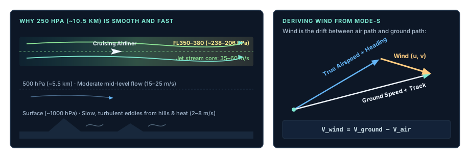
Fig. 2: Upper-air winds near cruising altitude and the velocity vectors used to estimate wind from aircraft data.
Why do so few aircraft produce a plausible map?
At first glance, building a regional wind map from 15 or 20 aircraft looks like guesswork. Actually, the solver needs only three valid vectors to start, but the result becomes more informative as additional aircraft cross the region. At cruising altitude, the airflow is well above any hills, obstacles and buildings that disturb surface winds, and large-scale weather systems can extend across hundreds of kilometres. That makes a smooth regional flow a useful starting point. Aircraft near a jet stream or a trough can then pull the field towards the winds they observe.
Why not just interpolate?
With 15 to 25 aircraft wind vectors over the region, simple distance-weighted interpolation would easily fill the gaps. Instead of redrawing a static average on every update, I wanted a flow field that keeps moving on its own while incoming aircraft data gently steer it.
It is a fun experiment rather than a benchmark against interpolation: the aircraft anchor the field where they fly, and the fluid solver smoothly connects the spaces in between.
How the backend works
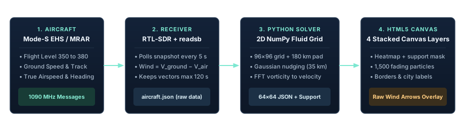
Fig. 3: From aircraft observations to an animated wind map in the browser.
The backend reads a local readsb aircraft snapshot about every five seconds. It keeps aircraft between 35,000 and 38,000 feet with sufficiently fresh positions and the required Mode-S airspeed and heading fields (standard ADS-B broadcasts alone do not include them). The wind estimate comes from ground speed and track minus true airspeed and true heading, expressed as eastward and northward velocities in metres per second.
The input is selective: not every aircraft supplies all the required fields, and the timing and quality checks can reject a candidate. The solver retains the latest accepted wind from each aircraft for at most two minutes and needs at least three aircraft to display a field.
Those observations feed a compact 2D fluid solver written in NumPy. It evolves vorticity, the local spin of the air, on a 96 × 96 grid covering Benelux and western Germany. A separate mean wind carries the overall flow. A fast Fourier transform (FFT) and a mathematical helper called a streamfunction turn the local spin back into smooth horizontal wind arrows.
The resulting field is incompressible: in this simplified 2D layer, air flows through the grid without piling up or disappearing. The streamfunction gives the wind field this property by construction.
The FFT grid is periodic: its opposite edges connect. A 180 km buffer around the displayed region moves those artificial boundaries away from the area of interest and reduces their influence.
Each aircraft creates a Gaussian area of influence with a scale of 35 km: its influence is strongest near the aircraft and fades with distance. Where the model wind differs from an aircraft estimate, a correction pulls the local flow towards that observation.
In the code, TAU_S is the 120-second relaxation time. denominator handles overlapping influences: it divides by their combined weight when that weight exceeds one, while keeping weak, isolated influences weak and avoiding division by zero.
denominator = np.maximum(1, weights.sum(axis=0))
east = np.array([row["east"] for row in items])[:, None, None]
north = np.array([row["north"] for row in items])[:, None, None]
force_u = np.sum(weights * (east - u), axis=0) / (denominator * TAU_S)
force_v = np.sum(weights * (north - v), axis=0) / (denominator * TAU_S)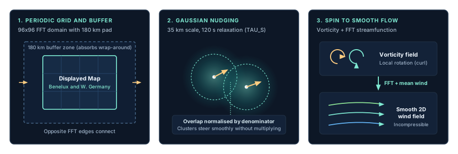
Fig. 4: How the 2D solver handles boundaries, overlapping aircraft influences and the conversion from local spin to a smooth wind field.
The solver takes the curl of this correction: it extracts the part that would make the local flow spin, then adds that rotational push to the vorticity field. The overall mean wind is adjusted separately. Viscosity and damping keep the experiment controlled as observations come and go.
This simplified 2D flow model turns scattered observations into a continuous picture. It has no vertical structure of its own, so the smooth flow between aircraft is the model’s reconstruction.
Rendering streamlines in HTML5 Canvas
The frontend is a single HTML file with four stacked <canvas> elements and no external JavaScript dependencies:
- Heatmap: Samples the 64 × 64 output grid and maps wind speed from 0 to 65+ m/s to a colour gradient. A support mask fades areas far from recent aircraft observations.
- Particles: Animates 1,500 particles through the modelled velocity field. Each particle leaves a short line segment; fading the previous frame with
destination-increates the trails. - Map: Draws country borders from local Natural Earth data and labels nearby cities.
- Observations: Overlays aircraft wind arrows for comparison with the calculated field.
The browser animates with requestAnimationFrame. Particle motion is deliberately accelerated so the flow’s direction and structure are easy to see.
What you see
When strong upper-level winds pass over the region, the map can show a fast-moving band of air above the much slower winds we experience at the surface. The arrows show the individual aircraft estimates; the colour and streamlines show how the 2D solver has combined them into a field.
For comparison, I can switch to GFS winds from Open-Meteo, select 250 hPa and look for similarities and differences. The two fields are independent: the aircraft-only solver runs entirely on aircraft winds.
Dark areas are just as important as bright ones: they indicate little recent aircraft coverage.
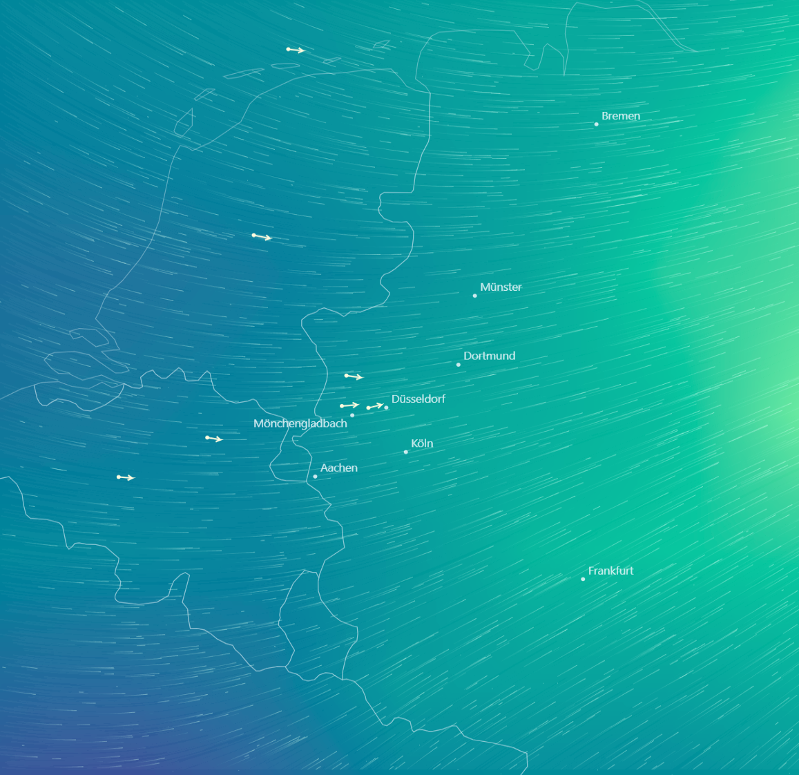
Fig. 5: The GFS comparison view at 250 hPa from Open-Meteo, overlaid with the same aircraft wind arrows for side-by-side orientation.
Lessons learned
- Keep observations and forecast models separate. A switch between the aircraft-only field and GFS makes it clear which data produced each picture.
- Adapt the time step. The solver subdivides updates according to wind speed and diffusion, rather than assuming one step is safe for every situation. Longer interruptions are reported and the amount of catch-up integration is bounded.
- Show the residual. The sidebar reports the wind-vector RMSE between the model and the aircraft winds used to steer it, as well as their actual altitude range. This measures the fit to those same observations; it is not an independent validation.
- Show where the data are. The support mask makes proximity to recent aircraft observations visible.
- Lightweight on hardware. In a 35-second benchmark, the backend produced a new field roughly every 5.3 seconds using about 10% of one CPU core. A separate measurement showed approximately 64 MB of RAM. An isolated test with a one-second target produced updates every 1.1 seconds at roughly 15% of one core, without errors.
The result is a small, live experiment: aircraft overhead supply the winds, NumPy evolves a flow field, and a browser turns it into a moving picture of the atmosphere above the home lab.
The source files are available here:
- Aircraft wind solver
- Map server and data ingestion
- Aircraft weather calculations
- HTML and Canvas frontend
The server requires NumPy, a Natural Earth borders GeoJSON file, and the extended readsb snapshot used in my lab, including its weather_provenance fields. Save the frontend as wind_map.html alongside the Python files to run it.