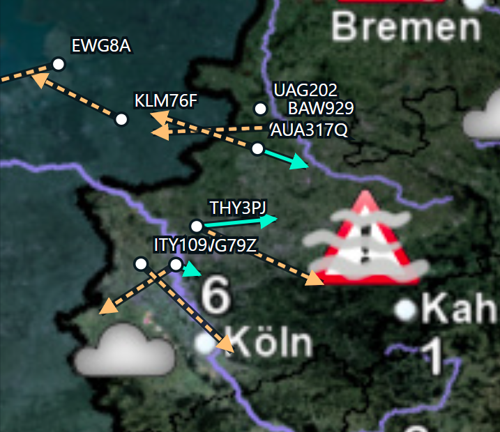
(Fig. 1: The local ADS-B / Mode-S helper app. Green arrows show winds derived from aircraft reports.)
Could aircraft passing overhead improve a local weather simulation?
This experiment originally started as a simple hardware benchmark. After upgrading my home-lab server with two Intel Xeon Gold 6238R processors (56 cores) from eBay, I compiled the Weather Research and Forecasting model (WRF) to see how well a real atmospheric simulation would scale on the new machine.
After the model was running, an idea came to my mind: could I feed live wind observations from my RTL-SDR USB stick (using ADS-B / Mode-S) into the simulation?
I quickly learned that commercial aviation already supplies professional weather models with upper-air data through programs like AMDAR, so the underlying principle is well established. However, I wanted to see what happens when I try that on a local scale with a basic home antenna.
As my receiver sits in western Germany near Düsseldorf Airport and the Rhine-Ruhr airspace, the dataset is naturally limited to traffic passing within local radio range. Working with the data also made an important constraint clear early on: commercial flights provide dense, reliable measurements almost exclusively at cruise altitude, around the 250 hPa pressure level (~10 km / 34,000 ft), rather than near the ground. (Note: This was also a lesson I learned. Meteorologists use hPa to describe heights, not feet or metres.)
Across four wind-only experiments, I tested a conservative baseline weight, increased the nudging strength, doubled the active time window, and finally upgraded both the receiver dongle and antenna to capture 35 times more records. The model clearly responds at cruise altitude, yet even with much better coverage, the improvement measured against holdout aircraft (aircraft whose observations were kept out of the nudging) remains small.
Background: How WRF and nudging work
WRF: A local weather model like WRF cannot start from an empty sky. Think of it like simulating a short stretch of a river. You need to know where the water is right now, and fresh water must keep flowing in from upstream. Global datasets like NOAA GFS supply both, and WRF calculates how the air moves from there.
Nudging: Nudging gives the simulated wind a gentle, temporary push toward the measured wind, rather than replacing it abruptly. If you force one spot to match a new wind speed all at once, you create artificial disturbances. Instead, nudging blends the measurement smoothly into the surrounding flow.
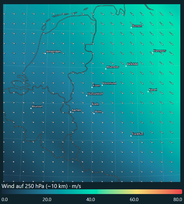
(Fig. 2: The unnudged control simulation showing wind at 250 hPa for 10 November 2026 at 10:00 CET.)
The idea: aircraft as moving atmospheric probes
Aircraft in flight broadcast motion parameters such as ground speed, track, true airspeed, and heading. Combining them gives the horizontal wind vector:
wind vector = ground-velocity vector - air-velocity vectorGround speed and track describe movement over the ground, whereas true heading and true airspeed describe movement through the surrounding air. Because cruise airspeeds are high, even a small heading error creates a noticeable error in the calculated wind. True airspeed and Mach number also allow an approximate temperature estimate, though for these four experiments I used wind only.
To apply this in WRF, the model compares its simulated wind at an aircraft’s position, altitude, and time against the observed wind, then adds a gentle corrective term proportional to that difference. A nudging coefficient controls how strongly this correction pulls, while weighting functions spread the adjustment smoothly across a nearby horizontal radius, a vertical layer, and a short time window.
The experiment setup
These were retrospective experiments: I recorded the aircraft data first, then replayed the same weather period with and without those observations.
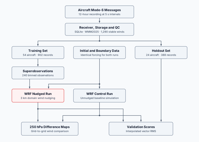
(Fig. 3: Processing and evaluation pipeline for Runs 1 to 3. Both WRF runs share identical initial and boundary data; only the nudged run receives the 240 training superobservations, while the 24 holdout aircraft evaluate both runs independently.)
The receiver runs locally and logs decoded messages into SQLite, where raw reports are grouped in space and time into superobservations (nearby reports combined into one representative observation). For Runs 1 to 3, WRF ran a nested setup over western Europe with a 9 km outer domain and a 3 km inner domain (where model grid points sit 3 km apart), covering 18 hours from 9 November 2026 18:00 UTC to 10 November 2026 12:00 UTC with hourly output. Observation nudging was applied only to the 3 km inner domain. Feedback from the inner domain to the outer domain was disabled, so the surrounding weather stayed identical. Each observation acts across a short symmetric time window around its timestamp.
The receiver runs locally and logs decoded messages into SQLite, where raw reports are grouped in space and time into superobservations (nearby reports combined into one representative observation). For Runs 1 to 3, WRF ran a nested setup over western Europe with a 9 km outer domain and a 3 km inner domain (where model grid points sit 3 km apart), covering 18 hours from 9 November 2026 18:00 UTC to 10 November 2026 12:00 UTC with hourly output. Observation nudging was applied only to the 3 km inner domain. Feedback from the inner domain to the outer domain was disabled, so the surrounding weather stayed identical. Each observation acts across a short symmetric time window around its timestamp.
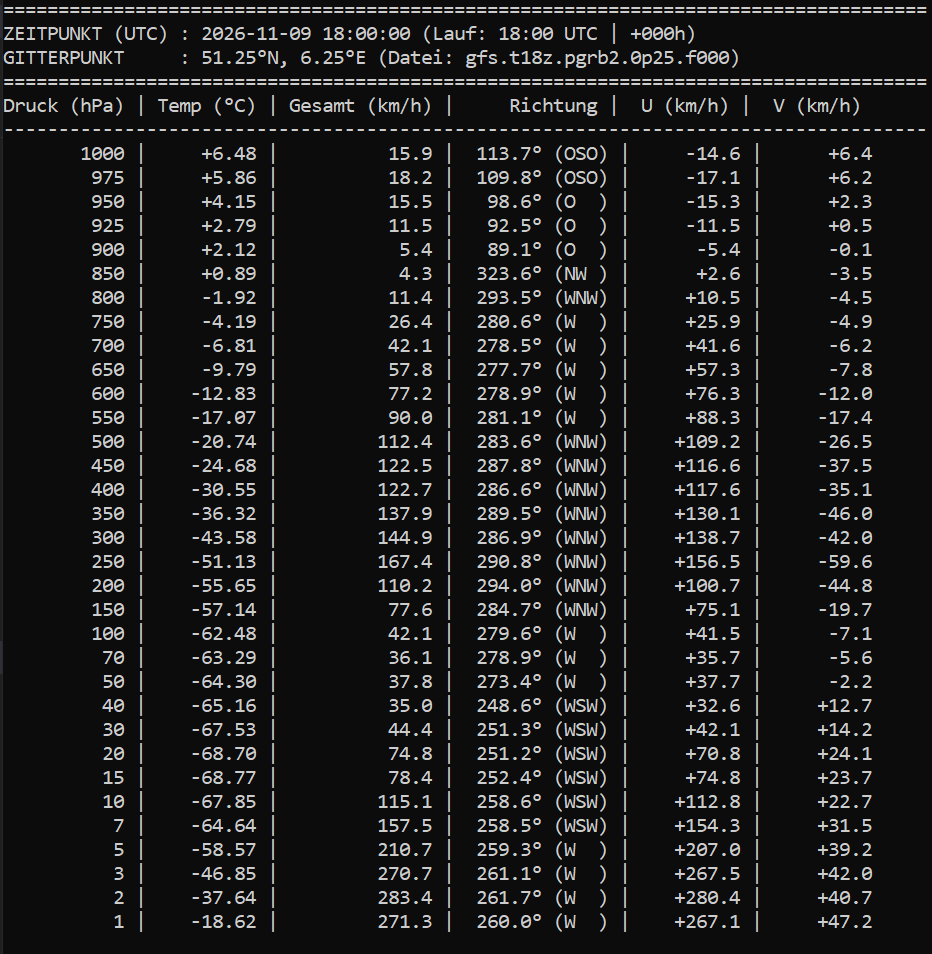
(Fig. 4: Vertical atmospheric profile from the GFS initial dataset at 51.25°N, 6.25°E for 9 November 2026 at 18:00 UTC, showing temperature, wind speed, direction, and east/north (U/V) components across pressure levels.)
To evaluate the simulations, simulated winds are compared directly against each aircraft report at its position, altitude, and time.
From a night of radio data to a candidate set
The initial overnight recording lasted 12 hours and sampled every five seconds:
| Recorded quantity | Count |
|---|---|
| Successful snapshots | 8,640 |
| Aircraft records | 15,648 |
| Aircraft identities | 371 |
| Wind candidates before strict screening | 13,815 |
| Stable wind candidates after screening | 1,290 |
Aircraft remain in range across many snapshots. Filtering out repeated, unstable, and maneuvering reports leaves 1,290 stable wind records from 78 aircraft. Of these, 98.4% are at or above 30,000 feet, making this primarily a cruise-level dataset.
This first recording did not store individual reception timestamps per Mode-S field, meaning airspeed, heading, and ground velocity could come from slightly different moments. Capturing per-field timestamps became a key improvement for Run 4.
The magnetic-heading correction
To subtract an aircraft’s airspeed from its ground velocity, both vectors must align with geographic true north. However, aircraft broadcast magnetic heading, which differs from true north and shifts slowly over time as Earth’s magnetic field drifts. At cruise speeds around 850 km/h, even a small angle error noticeably shifts the calculated wind vector.
The deployed decoder had still been using the older WMM2020 geomagnetic model even though the experiment took place in late 2026. Updating the decoder to WMM2025 shifted the derived wind vectors by a median of 0.76 m/s. That was worth fixing, though still small compared to the roughly 6 m/s median difference between aircraft winds and the unnudged control simulation.
Holding out entire aircraft
To avoid testing the model against another snapshot from the very same flight it just assimilated, I split the dataset by whole aircraft identities rather than individual rows. That left 902 training records from 54 aircraft and 388 holdout records from 24 different aircraft.
The 902 training records were thinned into 240 superobservations using 9 km horizontal, five-minute time, and 25 hPa pressure bins. Within each bin, each aircraft first contributes a median vector, and aircraft medians then receive equal weight so frequently sampled flights do not dominate. Runs 1 to 3 were evaluated against this 24-aircraft holdout set, while Run 4 used a separate holdout set from a new recording.
Run 1: Conservative baseline (3e-5 s⁻¹)
What was tested:
Run 1 served as a stability check to verify that real aircraft data would not destabilize the simulation. I enabled wind nudging on the 3 km domain with a very weak coefficient of 3e-5 s⁻¹. That corresponds to a relaxation timescale of roughly 9.3 hours, meaning the model is pulled only very gently toward each measurement during the few minutes an aircraft passes overhead.
How it was measured:
To see if the wind field actually improved, I compared the simulated winds against the actual aircraft measurements (calculating the root-mean-square vector error in m/s; lower is better). The evaluation is split into two groups:
- Training aircraft (54): A sanity check to verify that the assimilated observations actually moved the model.
- Holdout aircraft (24): The real test, checking whether the simulation also became more accurate for independent flights the model never saw.
| Evaluation set | Control error (RMS) | Nudged error (RMS) | Improvement versus matching control |
|---|---|---|---|
| Training aircraft (54) | 7.105 m/s | 7.065 m/s | 0.57% |
| Holdout aircraft (24) | 7.880 m/s | 7.864 m/s | 0.19% |
Result:
The pipeline ran end-to-end without numerical issues, confirming that the setup is stable. However, a nudging weight this conservative barely moved the needle, reducing the wind error on unseen holdout aircraft by just 0.19%.
What does a “0.2% improvement” actually mean?
It does not mean the simulation runs faster or predicts rain on the ground any better. It strictly measures wind accuracy at cruise altitude: how closely WRF’s simulated wind speed and direction match what real aircraft actually experienced.
Without nudging, WRF’s wind vectors differ from the holdout aircraft measurements by an average (RMS) of 7.88 m/s (~28 km/h), for example because the simulated jet stream is slightly shifted or off in speed. A 0.19% reduction shrinks that gap to 7.86 m/s. The simulation moved in the right direction, but by less than 0.02 m/s, a change far smaller than normal turbulence or aircraft sensor noise.
Run 2: Increasing the nudging coefficient to 1e-4 s⁻¹
After Run 1 showed that a weak weight barely moved the simulation, Run 2 tested whether increasing the 3 km wind nudging coefficient roughly threefold (from 3e-5 to 1e-4 s⁻¹, cutting the relaxation timescale from 9.3 to about 2.8 hours) would pull the model closer to independent aircraft winds. All other settings and the 240 training superobservations stayed identical:
| Evaluation set | Control error (RMS) | Nudged error (RMS) | Improvement versus matching control |
|---|---|---|---|
| Training aircraft (54) | 7.105 m/s | 6.976 m/s | 1.82% |
| Holdout aircraft (24) | 7.880 m/s | 7.831 m/s | 0.61% |
The stronger coefficient lowered holdout error by 0.61% relative to the control, up from 0.19% in Run 1 (a further 0.42% reduction over the first run). Individual aircraft results remained mixed (13 of the 24 holdout aircraft improved, 11 worsened), while individual wind components shifted by several metres per second on specific model levels.
Seeing the upper-air footprint
Comparing the 10 m surface wind maps initially showed almost no visible difference, which makes sense given that nearly all observations sit at cruise altitude. Plotting a difference map on the 250 hPa pressure surface (around 10 km above sea level) made the model response clearly visible:
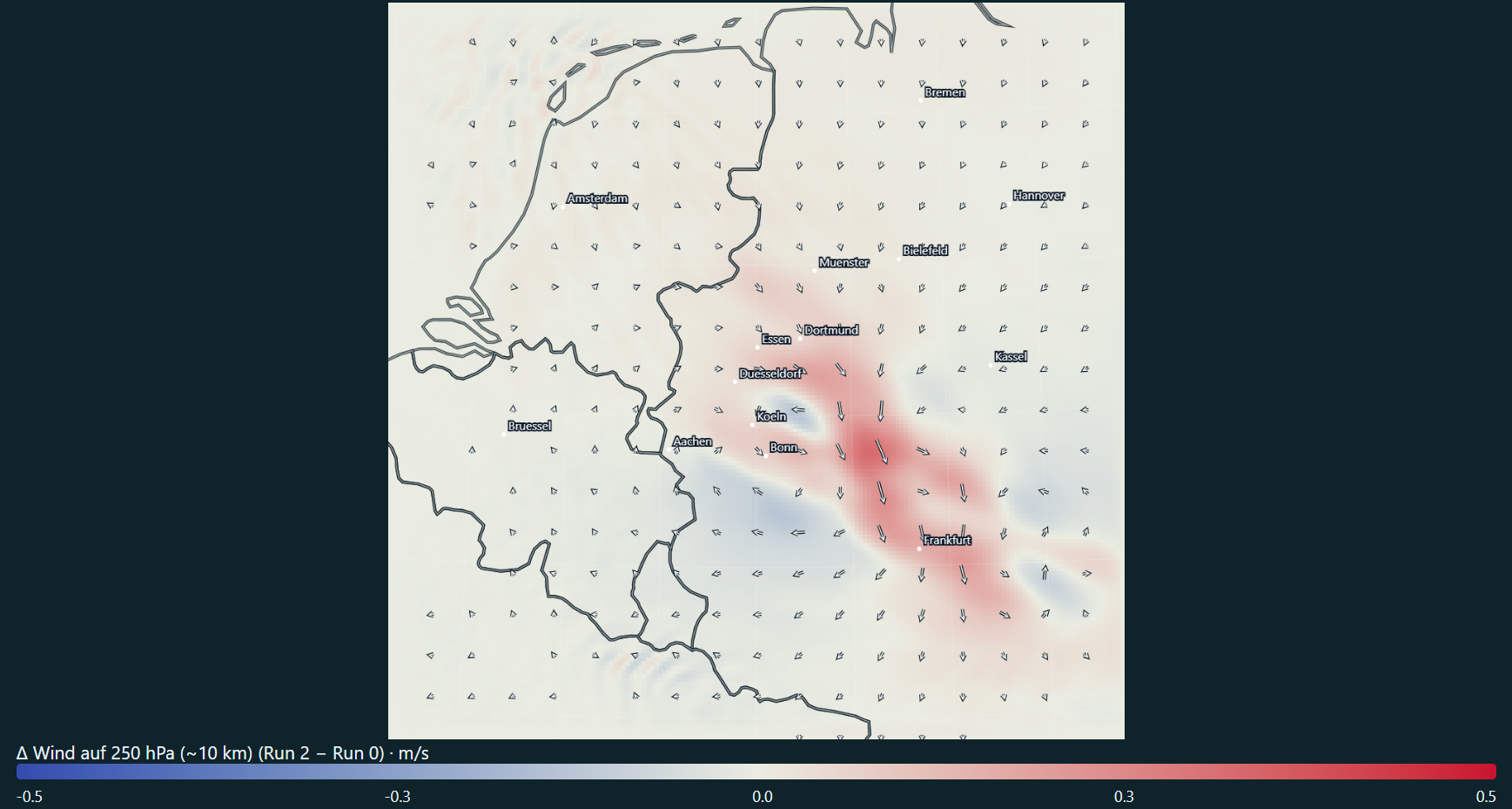
(Fig. 5: Wind changes at 250 hPa, approximately cruise altitude. Colors show the change in wind speed; arrows show the change in the wind vector, calculated as Run 2 minus the control. The color scale is fixed at -0.5 to +0.5 m/s.)
At 250 hPa, a coherent footprint appears: a band of accelerated wind extends from the Rhine-Ruhr region toward Frankfurt, flanked by smaller patches of slower wind. Difference arrows in the core point mostly south to southeast, showing the added wind adjustment rather than the actual wind direction. Across all 19 hourly maps, 250 hPa speed differences range from -0.216 to +0.325 m/s.
Run 2 confirmed that a stronger nudging weight triples the holdout improvement to 0.61% and leaves a clear, coherent wind footprint at cruise altitude, even though near-surface wind maps barely change.
Run 3: Doubling the time window
In the previous runs, each aircraft measurement only influenced the simulation for 15 minutes total (7.5 minutes before and after its timestamp). Because commercial flights pass overhead with empty gaps in between, Run 3 tested whether doubling that active window to ±15 minutes (30 minutes total) would bridge the pauses between flights and give each observation more time to steer the wind. The nudging coefficient stayed at 1e-4 s⁻¹:
| Evaluation set | Control error (RMS) | Nudged error (RMS) | Improvement versus matching control |
|---|---|---|---|
| Training aircraft (54) | 7.105 m/s | 6.929 m/s | 2.48% |
| Holdout aircraft (24) | 7.880 m/s | 7.821 m/s | 0.74% |
Keeping each measurement active twice as long pulled the simulation 2.48% closer to the training flights relative to the control, but added just 0.13% of extra improvement on the unseen holdout aircraft, bringing total holdout improvement to 0.74% (with 11 flights improving and 13 worsening compared to Run 2). Doubling the active time window produced very little additional benefit for independent flights.
Run 4: A new receiver, antenna, and 35x more data
With parameter tuning leveling off below 1% improvement, Run 4 tested whether sparse data coverage was the main bottleneck. I upgraded both the receiver dongle and antenna and recorded 24 hours from 11 November 2026 17:29 UTC to 12 November 17:29 UTC:
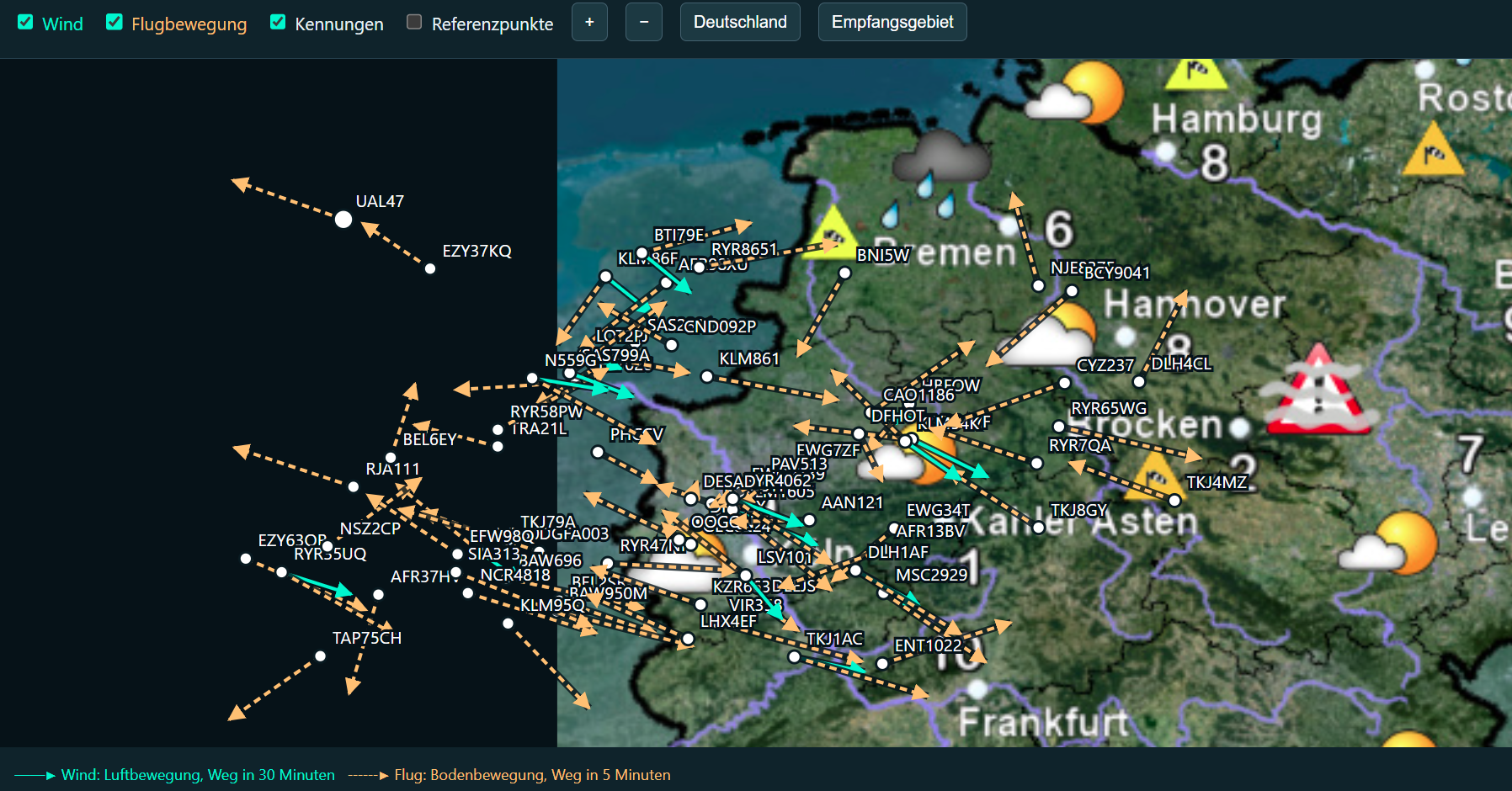
(Fig. 6: Live Mode-S reception with the upgraded dongle and antenna. Orange dashed arrows show 5-minute aircraft flight paths, while cyan arrows show derived 30-minute wind vectors spanning from the North Sea across western and northern Germany.)
| Recorded quantity | Original receiver setup | New dongle and antenna |
|---|---|---|
| Recording duration | 12 hours | 24 hours |
| Aircraft records | 15,648 | 543,191 |
| Aircraft identities | 371 | 2,502 |
| Derived wind candidates before WRF screening | 13,815 | 232,664 |
Doubling the recording duration with better hardware captured 35 times as many aircraft records and 6.7 times as many unique aircraft. The updated recorder also applied WMM2025 directly and stored per-field reception timestamps alongside the raw Mode-S messages.
I ran a matching 27-hour unnudged control (11 November 15:00 UTC to 12 November 18:00 UTC) and a paired nudged run using the Run 2 settings (1e-4 s⁻¹, ±7.5-minute half-window). After screening and binning, 518 training aircraft provided 12,390 superobservations. A separate set of 154 holdout aircraft (excluding all identities seen in the earlier recording) supplied 3,597 evaluation points:
| Evaluation set | Control error (RMS) | Nudged error (RMS) | Improvement versus matching control |
|---|---|---|---|
| Training aircraft (518) | 8.062 m/s | 7.943 m/s | 1.47% |
| Holdout aircraft (154) | 7.989 m/s | 7.930 m/s | 0.73% |
103 of the 154 holdout aircraft (67%) showed a lower wind error in the nudged run, with the clearest gains appearing above 30,000 feet.
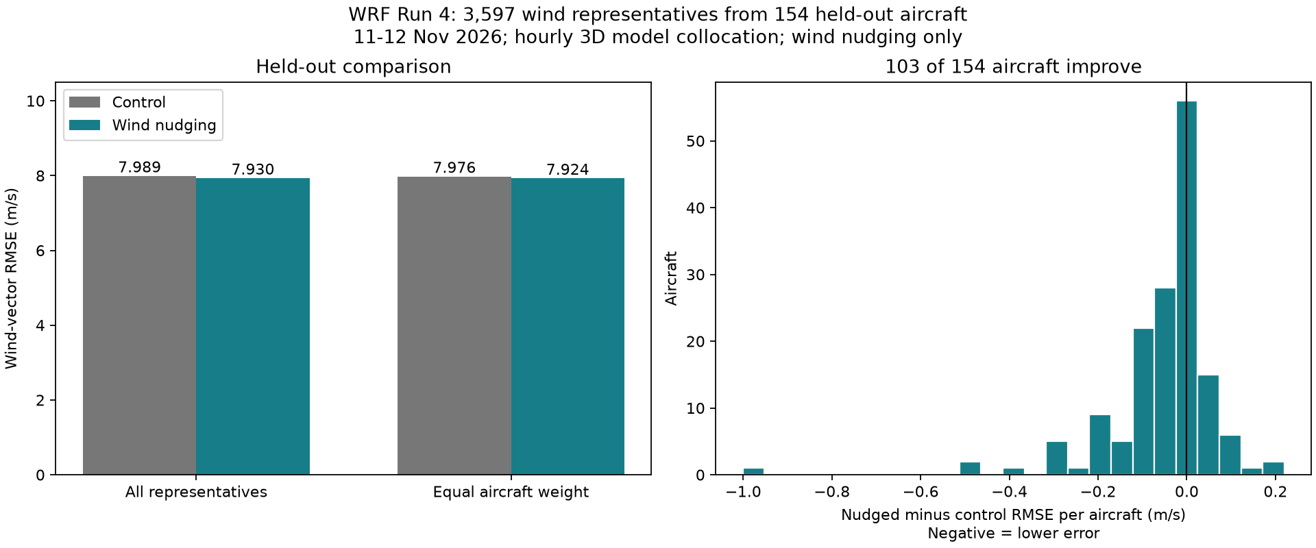
(Fig. 7: Run 4 evaluated against the 154 holdout aircraft. Left: wind-vector RMS error for control vs. nudged runs. Right: per-aircraft error change; negative values indicate closer agreement.)
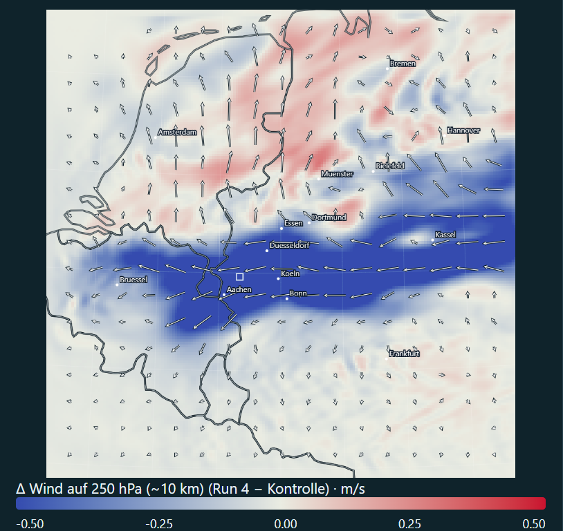
(Fig. 8: Wind changes at 250 hPa for Run 4 minus the matching control. With 35 times more records from the upgraded receiver, the nudging footprint spans most of the inner domain, showing a west-to-east band of reduced wind speeds across Belgium and western Germany alongside a northward shift over the Netherlands.)
Thirty-five times as many records. A wind adjustment stretching across most of the map. Closer agreement for two-thirds of the holdout aircraft. And still, the overall error fell by just 0.73%.
What likely limits the gains?
- The correction travels with the wind: At 35 m/s, air travels about 125 km in an hour. A correction introduced over western Germany moves downstream and can leave the inner domain within a few hours. Meanwhile, the surrounding model keeps supplying weather that has not received those aircraft corrections.
- A longer window does not create a fresh measurement: The observation stays tied to its recorded location. At the same wind speed, air travels more than 60 km during a 30-minute window. Extending that window keeps pulling at the old location; it does not follow the measured air downstream.
- Wind is only one part of the atmosphere: Wind, pressure, and temperature have to fit together. Wind-only nudging changes one part directly and leaves the model to readjust the others. More wind reports therefore do not automatically produce a better-balanced atmosphere.
What I take away from the experiment
What works
An inexpensive local ADS-B receiver and antenna can reliably supply upper-air wind estimates from commercial air traffic. The entire pipeline runs smoothly from radio reception and per-field timing through WMM2025 heading correction and superobservation binning into WRF, producing a visible wind response at cruise altitude and modest gains on holdout flights.
What would unlock larger improvements
Looking across all four runs, getting substantially more value out of local aircraft data points in three directions:
- Better observations: Storing and auditing raw Mode-S radio messages directly would allow tighter consistency checks on field timing, airspeed, and heading so noisy reports are filtered out before nudging.
- More vertical information: Capturing climbing and descending flights near airports alongside Mode-S derived temperatures would provide data across multiple altitudes instead of relying almost exclusively on cruise-level wind.
- Better-matched assimilation: Narrowing the vertical spread so cruise-level measurements do not smear across several kilometres of altitude, and adjusting temperature and pressure alongside wind, would let the model integrate the measurements more cleanly.
The receiver upgrade solved the data-volume problem. Turning those observations into a substantially better weather simulation takes more than collecting more aircraft.
Further reading
- NOAA/NCEI World Magnetic Model
- WRF User’s Guide: observation-nudging namelist options
- Stauffer & Seaman (1990): Use of Four-Dimensional Data Assimilation in a Limited-Area Mesoscale Model (Monthly Weather Review)
- de Haan (2011): High-resolution wind and temperature observations from aircraft tracked by Mode-S air traffic control radar (JGR Atmospheres)